Content
- Introduction
- The basic math formula for the Rosenblatt Perceptron
- Take a linear combination of input values
- Oooh, hold your horses! You say what? A ‘Vector’ ?
- Linearely seperable features
- A Hyper-what?
- Linear Sepera-what-ility ?
- As I was saying: Linearily seperable …
- The Heaviside Step Function
- Learning the weights
- Convergence of the learning rule.
- Wrap up
- What is wrong with the Rosenblatt perceptron?
- References
Introduction
A lot of articles introduce the perceptron showing the basic mathematical formulas that define it, but without offering much of an explanation on what exactly makes it work.
And surely it is possible to use the perceptron without really understanding the basic math involved with it, but is it not also fun to see how all this math you learned in school can help you understand the perceptron, and in extension, neural networks?
I also got inspired for this article by a series of articles on Support Vector Machines, explaining the basic mathematical concepts involved, and slowly building up to the more complex mathematics involved. So that is my intention with this article and the accompaning code: show you the math envolved in the preceptron. And, if time permits, I will write articles all the way up to convolutional neural networks.
Of course, when explaining the math, the question is: where do you start and when do you stop explaining? There is some math involved that is rather basic, like for example what is a vector?, what is a cosine?, etc… I will assume some basic knowledge of mathematics like you have some idea of what a vector is, you know the basics of geometry, etc… My assumptions will be arbitraty, so if you think i’m going too fast in some explanations just leave a comment and I will try to expand on the subject.
So, let us get started.
Disclaimer
This article is about the math involved in the perceptron and NOT about the code used and written to illustrate these mathematical concepts. Although it is not my intention to write such an article, never say never…
Setting some bounds
A perceptron basically takes some input values, called “features” and represented by the values $x_1, x_2, ... x_n$ in the following formula, multiplies them by some factors called “weights”, represented by $w_1, w_2, ... w_n$, takes the sum of these multiplications and depending on the value of this sum outputs another value $o$:
There are a few types of perceptrons, differing in the way the sum results in the output, thus the function $f()$ in the above formula.
In this article we will build on the Rosenblatt Perceptron. It was one of the first perceptrons, if not the first. During this article I will simply be using the name “Perceptron” when referring to the Rosenblatt Perceptron
We will investigate the math envolved and discuss its limitations, thereby setting the ground for the future articles.
The basic math formula for the Rosenblatt Perceptron
So, what the perceptron basically does is take some linear combination of input values or features, compare it to a threshold value $b$, and return 1 if the threshold is exceeded and zero if not.
The feature vector is a group of characteristics describing the objects we want to classify.
In other words, we classify our objects into two classes: a set of objects with characteristics (and thus a feature vector) resulting in in output of 1, and a set of objects with characteristics resulting in an output of 0.
If you search the internet on information about the perceptron you will find alternative definitions which define the formula as follows:
We will see further this does not affect the workings of the perceptron
Lets digg a little deeper:
Take a linear combination of input values
Remember the introduction. In it we said the perceptron takes some input value $[x_1, x_2, ..., x_i, ..., x_n]$, also called features, some weights $[w_1, w_2, ..., w_i, ..., w_n]$, multiplies them with each other and takes the sum of these multiplications:
This is the definition of a Linear Combination: it is the sum of some terms multiplied by constant values. In our case the terms are the features and the constants are the weights.
If we substitute the subscript by a variable $i$, then we can write the sum as
This is called the Capital-sigma notation, the $\sum$ represents the summation, the subscript $_{i=1}$ and the superscript $^{n}$ represent the range over which we take the sum and finally $w_ix_i$ represents the “things” we take the sum of.
Also, we can see all $x_i$ and all $w_i$ as so-called vectors:
In this, $n$ represents the dimension of the vector: it is the number of scalar elements in the vector. For our discussion, it is the number of characteristics used to describe the objects we want to classify.
In this case, the summation is the so-called dot-product of the vectors:
About the notation: we write simple scalars (thus simple numbers) as small letters, and vectors as bold letters. So in the above $x$ and $w$ are vectors and $x_i$ and $w_i$ are scalars: they are simple numbers representing the components of the vector.
Oooh, hold your horses! You say what? A ‘Vector’ ?
Ok, I may have gone a little too fast there by introducing vectors and not explaining them.
Definition of a Vector
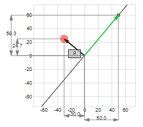
To make things more visual (which can help but isn’t always a good thing), I will start with a graphical representation of a 2-dimensional vector:
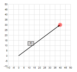
The above point in the coordinate space $\mathbb{R}^2$ can be represented by a vector going from the origin to that point:
We can further extend this to 3-dimensional coordinate space and generalize it to n-dimensional space:
In text (from Wikipedia):
A (Euclidean) Vector is a geometric object that has a magnitude and a direction
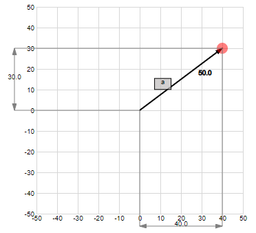
The Magnitude of a Vector
The magnitude of a vector, also called its norm, is defined by the root of the sum of the squares of it’s components and is written as $\lvert\lvert{\mathbf{a}}\lvert\lvert$
In 2-dimensions, the definition comes from Pythagoras’ Theorem:
Extended to n-dimensional space, we talk about the Euclidean norm:
Try it yourself:
Vector Magnitude interactive
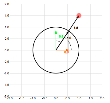
The Direction of a Vector
The direction of a 2-dimensional vector is defined by its angle to the positive horizontal axis:
This works well in 2 dimensions but it doesn't scale to multiple dimensions: for example in 3 dimensions, in what plane do we measure the angle? Which is why the direction cosines where invented: this is a new vector taking the cosine of the original vector to each axis of the space.
We know from geometry that the cosine of an angle is defined by:
So, the definition of the direction cosine becomes
This direction cosine is a vector $\mathbf{v}$ with length 1 in the same direction as the original vector. This can be simply determined from the definition of the magnitude of a vector:
This vector with length 1 is also called the *unit vector*.
Try it yourself:
Vector Direction interactive
Operations with Vectors
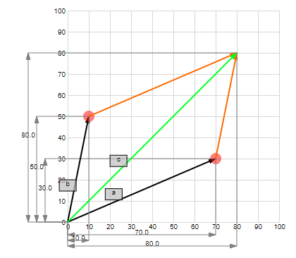
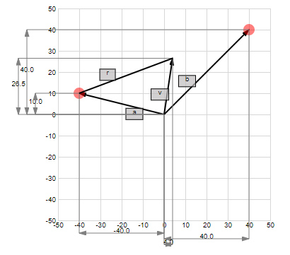
Sum and difference of two Vectors
Say we have two vectors:
The sum of two vectors is the vector resulting from the addition of the components of the orignal vectors.
Try it yourself:
Sum of vectors interactive
The difference of two vectors is the vector resulting from the differences of the components of the original vectors:
Try it yourself:
Difference of vectors interactive
Scalar multiplication
Say we have a vector $\mathbf{a}$ and a scalar $\lambda$ (a number):
A vector multiplied by a scalar is the vector resulting of the multiplication of each component of the original vector by the scalar:
Try it yourself:
Scalar Multiplication for vectors interactive
Dot product
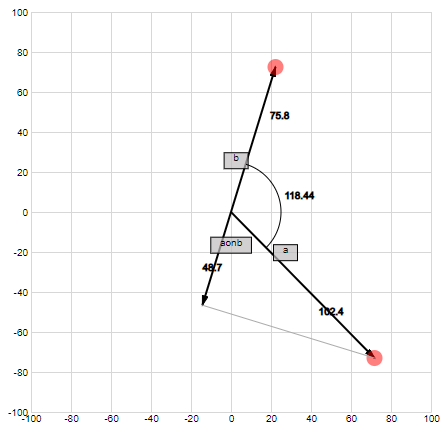
The dot-product is the scalar (a real number) resulting of taking the sum of the products of the corresponding components of two vectors:
Geometrically, this is equal to the multiplication of the magnitude of the vectors with the cosine of the angle between the vectors:
There are several proofs for this, which I will not repeat here. The article on SVM’s has one, and this article on the dot-product also contains a very understadable proof.
From this last definition we can make two important assertions.
First, if, for two vectors with a magnitude not zero, the dot product is zero, then those vectors are perpendicular. Because the magnitude of the vectors is not zero, the dot product can only be zero if the $cos(\alpha)$ is zero. And thus if the angle $\alpha$ between the vectors is either 90 or -90 degrees. And thus only if the two vectors are perpendicular. (Try it out in the interactive example below!)
Second, if one of the two vectors has a magnitude of 1, then the dot product equals the projection of the second vector on this unit vector. (Try it out in the interactive example below!). This can also easily be seen:
Try it yourself:
Dot Product interactive
The dot product is commutative:
Try it yourself:
Dot Product commutativity interactive
The dot product is distributive:
Try it yourself:
Dot Product distributivity interactive
The scalar multiplication property:
Okay, now you know what a Vector is. Let us continue our journey.
Linearely seperable features
So, we where saying: The sum of the products of the components of the feature and weight vector is equal to the Dot-product.
The perceptron formula now becomes:
Remember what we did originally: we took a linear combination of the input values $[x_1, x_2, ..., x_i, ..., x_n]$ which resulted in the formula:
You may remember a similar formula from your mathematics class: the equation of a hyperplane:
Or, with dot product notation:
So, the equation $\mathbf{w} \cdot \mathbf{x} > b$ defines all the points on one side of the hyperplane, and $\mathbf{w} \cdot \mathbf{x} <= b$ all the points on the other side of the hyperplane and on the hyperplane itself. This happens to be the very definition of “linear seperability”
Thus, the perceptron allows us to seperate our feature space in two convex half spaces.
A Hyper-what?
Let us step back for a while: what is this hyperplane and convex half spaces stuff?
Hyperplanes in one dimension: the equation of a line
A line through the origin
Never mind this hyperplane stuff. Let’s get back to 2-dimensional space and write the equation of a line as most people know it:
Let us even simplify this more and consider just:
Now, if we fix the values for $a$ and $b$ and solve the equation for various $x$ and $y$ and plot these values we see that the resulting points are all on a line.
If we consider $a$ and $b$ as the components of a vector $\mathbf{l}$, and $x$ en $y$ as the components of a vector $\mathbf{p}$, then the above is the dot product:
Then:
So, how come that setting our dot product to zero in two dimensions appears to be a line through the origin?
Remember that when we discussed the dot product, we came to the conclusion that if the dot product is zero for two vectors with magnitude not zero, then those vectors need to be perpendicular. So, if we fix the coordinates of the vector $\mathbf{l}$, thus fix the values $a$ and $b$, then the above equation resolves to all vectors perpendicular to the vector $\mathbf{l}$, which equals to all points on the line perpendicular to the vector $\mathbf{l}$ and going through the origin.
So, vector $\mathbf{l}$ determines the direction of the line: the vector is perpendicular to the direction of the line.
Try it yourself:
A line through the origin interactive
A line at some distance from the origin
Above, we simplified our equation resulting in the equation of a line through the origin. Let us consider the full equation again:
Rearranging a bit:
And replacing $-c$ with $d$:
Here also, we can consider replacing this with the dot product of vectors:
Then:
We can “normalize” this equation by dividing it through the length of $\mathbf{l}$, resulting in the dot product of the unit vector in the direction of $\mathbf{l}$: $\mathbf{u}$ and the vector $\mathbf{p}$:
And as seen above when discussing the dot product, this equals the magnitude of the projection of vector $\mathbf{p}$ onto the unit vector in the direction of $\mathbf{l}$. So, the above equation gives all vectors whose projection on the unit vector in the direction of $\mathbf{l}$ equals $d/{\lvert\lvert{\mathbf{l}}\lvert\lvert}$
This equals all vectors to points on the line perpendicular to $\mathbf{l}$ and at a distance $d/{\lvert\lvert{\mathbf{l}}\lvert\lvert}$ from the origin.
Try it yourself:
A line at some distance from the origin interactive
Extending to 3-dimensional space: equation of a plane
Again, through vectors:
If we consider the components $a$, $b$ and $c$ as a vector $\mathbf{m}$, and $x$, $y$ and $z$ as a vector $\mathbf{p}$, then the above is the dot product:
Then:
Again, if the dot product is zero for two vectors with magnitude not zero, then those vectors need to be perpendicular. So, if we fix the coordinates of the vector $\mathbf{m}$, thus fix the values $a$, $b$ and $c$, then the above equation resolves to all vectors perpendicular to the vector $\mathbf{m}$, which equals to all points in the plane perpendicular to the vector $\mathbf{m}$ and going through the origin.
A similar line of thought can be followed for the equation:
Here also, we can consider replacing this with the dot product of vectors:
Normalizing by dividing through the length of $\mathbf{m}$, with $\mathbf{u}$ being the unit vector in the direction of $\mathbf{m}$:
And as seen above when discussing the dot product, this equals the magnitude of the projection of vector $\mathbf{p}$ onto the unit vector in the direction of $\mathbf{m}$. So, the above equation gives all vectors whose projection on the unit vector in the direction of $\mathbf{m}$ equals $d/\lvert\lvert{\mathbf{m}}\lvert\lvert$
This equals all vectors to points in the plane perpendicular to $\mathbf{m}$ and at a distance $d/\lvert\lvert{\mathbf{m}}\lvert\lvert$ from the origin.
Extending to n-dimensional space: equation of a hyper-plane
In 3-dimensional space, we defined the equation of a plane as:
If we use the symbols we are customed to in our discussion of the percpetron rule, we can write:
This may be a bit confusing, but the $b$ in this last equation has nothing to do with the $b$ in the first equation
If we extend this to multiple dimensions, we get:
In multi-dimensional space we talk about hyper-planes: like a plane is a line in 3-dimensional space, a hyper-plane is a plane n multi-dimensional space.
Linear Sepera-what-ility ?
Ok, lets go back to the definition of the perceptron:
So, we output 1 if the dot product of the feature vector $\mathbf{x}$ and weight vector $\mathbf{w}$ is larger then $b$, and zero $\text{otherwise}$. But what is $\text{otherwise}$ ?
Well $\text{otherwise}$ is:
Ah, equal to or less then $b$. We know the equal to part, that is our above hyper-plane.
So what remains is the less than part
It just so happens the inequality equations define two so called half-spaces: one half space above the hyper-plane and one half-space below the hyper-plane.
Linear separability and half-spaces
Let us again take the equation of a hyperplane:
This hyperplane seperates the space $\mathbb{R}^n$ in two convex sets of points, hence the name half-space.
One half-space is represented by the equation
The other by
Let us analize the first equation. First, convert it to a vector representation:
Normalizing:
So, the geometric interpretation is the set of all vectors to points with a projection on the unit vector in the direction of the weight vector $\mathbf{w}$ larger then some constant value $\frac{b}{\lvert\lvert{\mathbf{w}}\lvert\lvert}$.
A similar reasoning can be made for the equation $\mathbf{w} \cdot \mathbf{x} < b$ : it results in the set of vectors to points with a projection on the unit vector in the direction of the weight vector $w$ smaller then some constant value $\frac{b}{\lvert\lvert{\mathbf{w}}\lvert\lvert}$.
We can imagine these two sets as being the set of all points on either one side or the other side of the hyper-plane.
These half spaces are also convex.
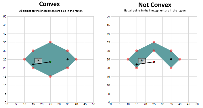
The definition of convex goes as follows (from Wikipedia):
in a Euclidean space, a convex region is a region where, for every pair of points within the region, every point on the straight line segment that joins the pair of points is also within the region.
Mathematically this can be more rigourously be described as:
A set $\mathbf{C}$ in $\mathbf{S}$ is said to be convex if, for all points $A$ and $B$ in $\mathbf{C}$ and all $\lambda$ in the interval $(0, 1)$, the point $(1 − {\lambda})A + {\lambda}B$ also belongs to $C$.
The equation $(1 − {\lambda})A + {\lambda}B$ is actually the equation of a line segment between points $A$ and $B$. We can see this from following:
Let us define two points in the multi-dimensional space:
Then a line segment going from point $A$ to point $B$ can be defined as:
with $\vec{OA}$ being the vector going from the origin $O$ to point $A$ and $\vec{AB}$ the vector going from point $A$ to point $B$. $\lambda$ is in the interval (0, 1)
This is simply the addition of the vector $\mathbf{a}$ with a part of the vector going from point $A$ to point $B$
Try it yourself:
Line segment interactive
We know from the section on vector math above that the vector going from $A$ to $B$ is equal to $\mathbf{b}-\mathbf{a}$ and thus we can write:
Now we can proof the half spaces separated by the hyper-plane are convex:
Let us consider the upper half plane. For any two vectors $\mathbf{x}$, $\mathbf{y}$ in that half space we have:
If the half space is convex, then each point resulting from the equation
must belong to the half space, which is equal to saying that every point on the line segment between the endpoints $X$ and $Y$ of the vectors must belong to the half space.
Substituation in the equation of the half space gives:
Then, by the distributive and scalar multiplication properties of the dot product we can re-arrange to:
Since we now that $0 < {\lambda} < 1$ and $\mathbf{w} \cdot \mathbf{x} > d$ and also $\mathbf{w} \cdot \mathbf{y} > d$ then the above inequality must also hold true. And thus we have proven that the half space is indeed convex.
Try it yourself:
Convex interactive
Not Convex interactive
As I was saying: Linearily seperable …
Thus, getting back at our formula for the preceptron:
We can now see how this formula divides our feature-space in two convex half spaces. Mind the word convex here: it does not just divide the feature space in two subspaces, but in two convex subspaces.
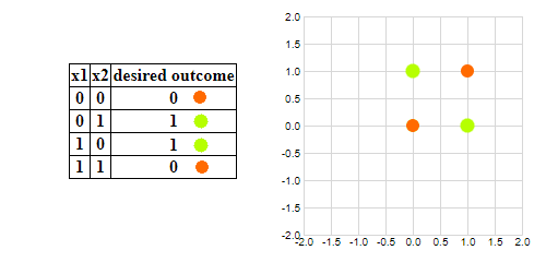
This means that we cannot seperate feature points into classes that are not convex. Visually in two-dimensional space, we cannot seperate features like this:
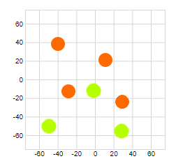
If you’ve been reading about the perceptron allready, you may have read about the fact that it cannot solve the XOR problem: it cannot seperate the inputs according to the XOR function. That is exactly because of the above: the outcome is not convex, hence is not linearily seperable.
If you search the internet for the formula of the Rosenblatt perceptron, you will also find some in which the factor $b$ is no longer present. What happened to it? Some re-arrangement of the components of the addition make it end up in the dot product:
Now, we can define $b' = -b$
Finally, we can take the factor 1 inside the feature vector by defining $x_0 = 1$ and $b'$ inside the weight vector by defining $w_0 = b'$. This lets us write:
And by taking $w_0$ and $x_0$ inside the vector:
We can now write:
So we have a function which classifies our features into two classes by multiplying them with a weight and if the result is positive assigns them a label “1” and “0” otherwise.
Further in the article I will leave the accent of the vectors and just write $\mathbf{w}$ and $\mathbf{x}$ which have the $w_0$ and $x_0$ included.
Try it yourself:
Perceptron math interactive
This assigning them a label “1” and “0” otherwise is the definition of the Heaviside Step Function.
The Heaviside Step Function
The Heaviside step function is also called the unit step function and is given by:
If you search the internet for the definition of the Heaviside step function, you may find alternative definitions which differ from the above on how the result of the function is defined when $x=0$
The Heaviside step function is discontinuous. A function $f(x)$ is continuous if a small change of $x$ results in a small change in the outcome of the function. This is clearly not the case for the Heaviyside step function: if at 0 and moving to the negative side then the function outcome changes suddenly from 1 to 0.
I will not elaborate much more on this function not being continuous because it is not important for the discussion at hand. In a next article, when we discuss the ADALINE perceptron, I will get back to this.
Learning the weights
We’ve covered a lot about how the perceptron classifies the features in two linearily seperable classes using the weight vector. But the big question is: if we have some samples of features for which we know the resulting class, how can we find the weights so that we can also classify unknown values of the feature vector? Or, how can we find the hyperplane sepeating the features?
This is where the perceptron learning rule comes in.
The perceptron learning rule
First, we define the error $e$ as being the difference between the desired output $d$ and the effective output $o$ for an input vector $\mathbf{x}$ and a weight vector $\mathbf{w}$:
Then we can write the learning rule as:
In this $\mathbf{w}_{i+1}$ is the new weight vector, $\mathbf{w}_{i}$ is the current weight vector and $e$ is the current error. We initialize the weight vector with some random values, thus $\mathbf{w}_0$ has some random values. You will find similar definitions of the learning rule which also use a learning rate factor. As we will show later when we proof the convergence of the learning rule this factor is not really necessary. That is why we leave it out here.
Why does this work? First, let us analyse the error function:
As stated before, in this $d$ and $o$ are resp. the desired output and the effective output of the perceptron. We know from the definition of the preceptron that its output can take two values: either 1 or 0. Thus the error function can take following values:
| prediction | desired (d) | effective (o) | e |
|---|---|---|---|
| correct | 1 | 1 | 0 |
| correct | 0 | 0 | 0 |
| wrong | 0 | 1 | -1 |
| wrong | 1 | 0 | 1 |
From the above we can see that
- We only change the weight vector $\mathbf{w}$ if the prediction made by the perceptron is wrong, because if it is correct the error amounts to zero.
- If we incorrectly predict a feature to be above the hyperplane then the error is -1 and we subtract the feature vector from the weight vector.
- If we incorrectly predict a feature to be below the hyperplane then the error is 1 and we add the feature vector to the weight vector.
Let’s see what this gives geometrically. The following discussion gives an intuitive feel of what the learning algorithm does, but is by no means a mathematically rigourous discussion. We start with ignoring the threshold factor of the vectors: that is, we ignore $w_0$ and $x_0$.
So, we are left with the factors determining the direction of the seperating hyperplane. Let us now plot some examples and see what happens.
Case 1: Desired result is 0 but 1 was predicted
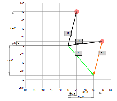
The error $e$ is -1, so we need to subtract the new feature vector from the current weight vector to get the new weight vector:
Remember that the weight vector is actually perpendicular to the hyperplane. The result of subtracting the incorrectly classified vector from the weight vector is a rotation of the separating hyperplane in the direction of the incorrectly classified point. In other words, we rotate the separating hyperplane in such a way that our newly learned point is closer to the half-space it belongs in.
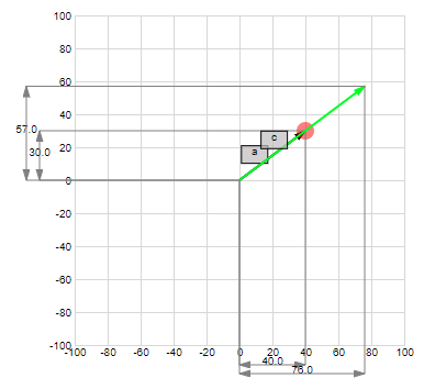
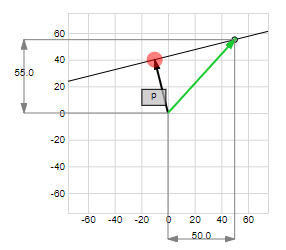
Case 2: Desired result is 1 but 0 was predicted
The error $e$ is 1, so we need to add the new feature vector to the current weight vector to get the new weight vector:
The result of adding the vector to the weight vector is a rotation of the separating hyperplane in the direction of the incorrectly classified point. In other words, we rotate the separating hyperplane in such a way that our newly learned point is closer to the half-space it belongs in.
Try it yourself:
Perceptron Learning interactive
Convergence of the learning rule.
The above gives an intuïtive feel of what makes the learning rule work, but is not a mathematical prove. It can be proven mathematically that the perceptron rule will converge to a solution in a finite number of steps if the samples given are linearily seperable.
Read that sentence again please. First, we talk about a finite number of steps but we don’t now what that number is up front. Second, this is only true if the samples given are linearly seperable. Thus, if they are not linearly seperable we can keep on learning and have no idea when to stop !!!
I will not repeat the proof here because it would just be repeating some information you can find on the web. Second, the Rosenblatt perceptron has some problems which make it only interesting for historical reasons. If you are interested, look in the references section for some very understandable proofs go this convergence. Of course, if anyone wants to see it here just leave a comment.
Wrap up
Basic formula of the Rosenblatt Perceptron
The basic formula classifies the features by weighting them into two seperate classes.
We have seen that the way this is done, is by comparing the dot product of the feature vector $\mathbf{x}$ and the weight vector $\mathbf{w}$ with some fixed value $b$. If the dot product is larger then this fixed value, then we classisify them info one class by assigning them a label 1, otherwise we put them into the other class by assigning them a label 0.
Behaviour of the Rosenblat Perceptron
Because the formula of the perceptron is basically a hyperplane, we can only classify things into two classes which are lineary seperable. A first class with things above the hyper-plane and a second class with things below the hyper-plane.
Formalising some things: a few definitions
We’ve covered a lot of ground here, but without using a lot of the lingo surrounding perceptrons, neural networks and machine learning in general. There was already enough lingo with the mathematics that I didn’t want to bother you with even more definitions.
However, once we start diving deeper we’ll start uncovering some pattern / structure in the way we work. At that point, it will be interesting to have some definitions which allow us to define steps in this pattern.
So, here are some definitions:
Feed forward single layer neural network
What we have now is a feed forward single layer neural network:
Neural Network
A neural network is a group of nodes which are connected to each other. Thus, the output of certain nodes serves as input for other nodes: we have a network of nodes. The nodes in this network are modelled on the working of neurons in our brain, thus we speak of a neural network. In this article our neural network had one node: the perceptron.
Single Layer
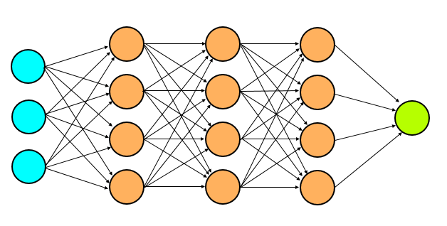
In a neural network, we can define multiple layers simply by using the output of preceptrons as the input for other perceptrons. If we make a diagram of this we can view the perceptrons as being organised in layers in which the output of a layer serves as the input for the next layer.
In this article we also have a single layer.
Feed Forward
This stacking of layers on top of each other and the output of previous layers serving as the input for next layers results in feed forward networks. There is no feedback of upper layers to lower layers. There are no loops. For our single perceptron we also have no loops and thus we have a feed forward network.
Integration function
The calculation we make with the weight vector w and the feature vector x is called the integration function. In the Rosenblatt perceptron the integration function is the dot-product.
Bias
The offset b with which we compare the result of the integration function is called the bias.
Activation function (transfer function)
The output we receive from the perceptron based on the calculation of the integration function is determined by the activation function. The activation function for the Rosenblatt perceptron is the Heaviside step function.
Supervised learning
Supervised learning is a type of learning in which we feed samples into our algorithm and tell it the result we expect. By doing this the neural network learns how to classify the examples. After giving it enough samples we expect to be able to give it new data which it will automatically classify correctly.
The opposite of this is Unsupervised learning in which we give some samples but without the expected result. The algorithm is then able to classify these examples correctly based on some common properties of the samples.
There are other types of learning like reïnforcement learning which we will not cover here.
Online learning
The learning algorithm of the Rosenblatt preceptron is an example of an online learning algorithm: with each new sample given the weight vector is updated;
The opposite of this is batch learning in which we only update the weight vector after having fed all samples to the learning algorithm. This may be a bit abstract here but we’ll clarify this in later articles.
What is wrong with the Rosenblatt perceptron?
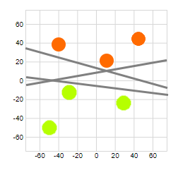
The main problem of the Rosenblatt preceptron is its learning algorithm. Allthough it works, it only works for linear seperable data. If the data we want to classify is not linearily seperable, then we do not really have any idea on when to stop the learning and neither do we know if the found hyperplane somehow minimizes the wrongly classified data.
Also, let’s say we have some data which is linearily seperable. There are several lines which can seperate this data:
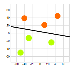
We would like to find the hyperplane which fits the samples best. That is, we would like to find a line similar to the following:
There are of course mathematical tools which allow us to find this hyperplane. They basically all define some kind of error function and then try to minimize this error. The error function is typically defined as a function of the desired output and the effective output just like we did above. The minimization is done by calculating the derivative of this error function. And herein is the problem for the Rosenblatt preceptron. Because the output is defined by the Heaviside Step function and this function does not have a derivative, because it is not continuous, we cannot have a matematically rigourous learning method.
If the above is gong a little to fast, don’t panic. In the next article about the ADALINE perceptron we’ll dig deeper into error functions and derivation.
References
Javascript libraries used in the Try it yourself pages
For the SVG illustrations I use the well known D3.js library
For databinding Knockout.js is used
Mathematical formulas are displayed using MathJax
Vector Math
The inspiration for writing this article and a good introduction to vector math: SVM - Understanding the math - Part 2
Some wikipedia articles on the basics of vectors and vector math:
Euclidean vector
Magnitude
Direction cosine
An understandable proof of why the dot-product is also equal to he product of the length of the vectors with the cosine of the angle between the vectors:
Proof of dot-product
Hyperplanes and Linear Seperability
Hyperplane
Linear separability
Two math stackexchange Q&A’s on the equation of a hyperplane:
Hyperplane equation intuition / geometric interpretation
Why is the product of a normal vector and a vector on the plane equal to the equation of the plane?
Convexity
Definition of convexity: Convex set
Discussing convexity, we also discussed Line segments: Line segment
Proving a half-plane is convex: How do I prove that half a plane is convex?
A more in depth discussion of convexity: Lecture 1 Convex Sets
Perceptron
Wikipedia on the perceptron: Perceptron
Another explanation of the perceptron: The Simple Perceptron
A Peceptron is a special kind of linear classifier
Following article as an interesting view on what they call the duality of input and weight-space: 3. Weighted Networks – The Perceptron
Perceptron Learning
Following article gives another intuitive explanation on why the learning algorithm works: Perceptron Learning Algorithm: A Graphical Explanation Of Why It Works
An animated gif of the perceptron learning rule: Perceptron training without bias
Convergence of the learning algorithm
This YouTube video presents a very understandable proof: Lec-16 Perceptron Convergence Theorem
A written version of the same proof can be found in this pdf: CHAPTER 1 Rosenblatt’s Perceptron By the way, there is much more inside that pdf then just the proof.